





A sieve analysis is a table of numbers; a size distribution model turns that table into a curve you can predict, blend and design with. The Gaudin-Schuhmann distribution is the simplest of these models, and for crushed products it is often startlingly good — two numbers describe the whole gradation.
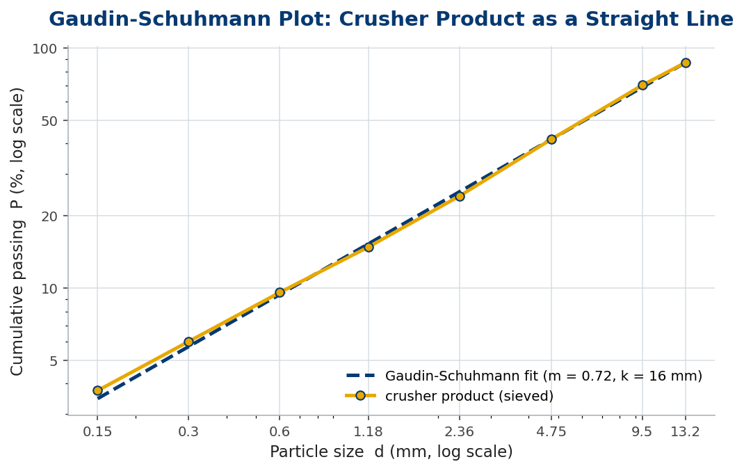
This article sets out the Gaudin-Schuhmann equation, shows why a crusher product plots as a straight line on log-log paper, and explains what its two parameters — the size modulus and the distribution modulus — tell you about the machine and the product.
The distribution
Gaudin and Schuhmann proposed that the cumulative fraction passing a size follows a simple power law:
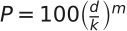
where  is the percent passing size
  ,
,  is the size modulus (the size at which the line projects to 100% passing, close to the top size) and
  is the distribution modulus (the slope). Take logarithms of both sides and the relationship is linear: a plot of
  against
  is a straight line of slope .
Worked example 1 — fitting the two parameters
Take two points off the sieve curve. Suppose 50% passes 4.0 mm and 10% passes 0.9 mm. The slope is

Then back out the size modulus from either point:  . With and in hand you can predict the passing at any sieve without testing it.
What the parameters mean
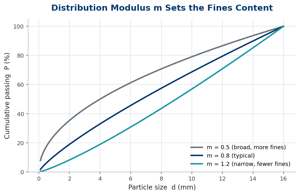
The distribution modulus is the more useful of the two. A low means a broad distribution with plenty of fines; a high means a narrow, more uniform product. Compression crushers (jaw, cone) typically give  –1.0, while impact crushers tend to run lower, producing more fines. The size modulus scales with the crusher setting — open the gap and the whole line shifts to coarser sizes.
| Parameter | Symbol | What it controls |
|---|---|---|
| Size modulus | k | top size; tracks crusher setting |
| Distribution modulus | m | slope; fines content and uniformity |
| Low m (<0.7) | — | broad, fines-rich (impact crushing) |
| High m (>1.0) | — | narrow, uniform product |
Worked example 2 — predicting the fines
With  and
and  , the fraction finer than 0.15 mm — the troublesome filler — is

Drop the modulus to  (a more impact-like product) and the same calculation gives about 6%, more than four times the filler. The model lets you see, before you buy the crusher, how its product character will load the downstream screens and washers.
In practice
Fit Gaudin-Schuhmann to every routine sieve analysis and trend the two parameters rather than a dozen sieve numbers — a drifting flags a worn setting, a falling flags worn liners making more fines. The model is a description, not a law: real products curl away from the straight line at the very top and very bottom, so fit it over the working range and do not extrapolate blindly. Where the fit is poor — broad or multi-modal feeds — reach for the Rosin-Rammler distribution instead, which adds a parameter and handles the tails better.
Common mistakes
- Reading the slope off the wrong axes. The straight line is on log-log paper; a semilog plot still curves.
- Extrapolating to the tails. Fit over the working sieves; the model bends away at top and bottom size.
- Forcing a fit on a bimodal feed. If two crushers or stockpiles mix, use Rosin-Rammler or model each mode.
When Gaudin-Schuhmann is not enough: Rosin-Rammler
The straight-line model is a gift when it works, but plenty of products refuse to lie straight — broad distributions, the coarse and fine tails, and feeds that mix two crushers all curve away from it. When they do, the Rosin-Rammler (also called Weibull) distribution is the usual next step:

where  is the percent retained above size ,
  is the characteristic size (the size at which 36.8% is retained) and
  is the spread parameter. Rosin-Rammler bends to follow the tails that Gaudin-Schuhmann misses, at the cost of being a little less intuitive to plot and fit.
The practical rule is to start simple. Fit Gaudin-Schuhmann first; if the points hug the line across the sieves you care about, you are done — two numbers, job finished. Only when the residuals fan out at the ends, or the fit is visibly poor, is the extra parameter of Rosin-Rammler earned. Reaching for the more complex model by default is a common waste of effort: most single-crusher products are Gaudin-Schuhmann to within the accuracy a plant ever needs.
Whichever model you fit, the discipline that makes it useful is the same: fit it to a clean sieve analysis, trend the parameters rather than the raw sieves, and read a change in a parameter as a change in the process. A drifting size modulus is the crusher opening up; a falling distribution (or spread) modulus is the product broadening as liners wear and make more fines. Two coefficients, watched over time, turn a stack of sieve tables into a live picture of crusher health — which is the whole reason to model a gradation rather than merely measure it.
The bottom line
Gaudin-Schuhmann,  , compresses a whole crusher gradation into a slope and a size: for the fines and uniformity, for the top size. On log-log axes it is a straight line you can read, fit and predict from.
Fit it to routine sieves, trend the two parameters as a health check on the crusher, and use it to forecast fines before they become a screening problem — two numbers doing the work of the whole table.
Frequently asked questions
What is the distribution modulus?
The slope m of the Gaudin-Schuhmann line on log-log axes. Low m means broad, fines-rich; high m means narrow and uniform.
How do I find k and m from a sieve test?
Take two points (size, %passing), compute m as the ratio of log-passing to log-size differences, then back out k from either point.
When should I use Rosin-Rammler instead?
When the product is broad or the tails matter — Rosin-Rammler adds a parameter and fits the coarse and fine ends better.
Key takeaways
- — a straight line on log-log axes for crushed products.
- m (slope) sets fines and uniformity; k (size modulus) tracks the crusher setting.
- Fit two sieve points to get both parameters, then predict any sieve.
- Trend m and k as a crusher health check; switch to Rosin-Rammler for broad feeds.
