






Every quote, every investment and every ‘should we run the night shift’ decision rests on one number: the cost to produce a tonne. Most plants carry it in their heads, vaguely. Built properly, the cost-per-tonne model is a short equation that separates the capital you have already spent from the cash you spend each tonne — and it reveals that utilisation, not any single line item, is usually the biggest lever you own.
This article assembles the model from its two halves, amortises the capital with the capital recovery factor, and shows how cost per tonne moves with how hard you run the plant.
The two halves
Cost per tonne is the annual cost divided by the annual tonnes. The annual cost is a fixed part (amortised capital plus standing costs) and a variable part that scales with production:

The variable cost  is energy, wear, consumables and the like — roughly constant per tonne. The fixed cost is spread over however many tonnes you make, which is why output matters so much.
| Symbol | Meaning | Units |
|---|---|---|
| Cfixed | Annual fixed cost (capital + standing) | Rs/yr |
| Tannual | Annual production | t/yr |
| cvar | Variable cost per tonne | Rs/t |
Amortising the capital
To turn a lump of capital into an annual cost, use the capital recovery factor, which converts a present capital sum into equal yearly payments over the asset life:
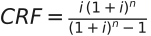
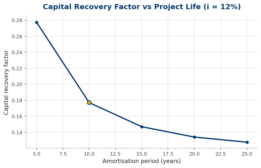
At  over
over  years,
  : a Rs 10 crore plant costs Rs 1.77 crore a year to own. Spreading it over more years lowers the annual bite, but with diminishing returns.
Worked example 1 — the cost per tonne
A Rs 10 crore plant ( Rs 1.77 cr/yr capital), plus Rs 0.23 crore/yr standing labour and overhead, has
  . Running 250 t/h for 4,000 hours gives
  . With
  :
:

Utilisation is the master lever
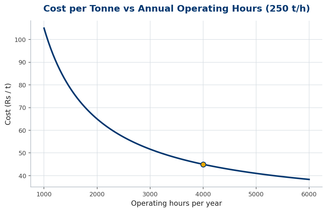
That Rs 20/t of fixed cost is not a constant — it is Rs 20 crore-worth of fixed cost divided by output. Run fewer hours and it balloons; run more and it shrinks toward the variable floor.
Worked example 2 — the utilisation penalty
Drop from 4,000 to 2,000 operating hours and annual output halves to 0.5 Mt. The fixed cost per tonne doubles to Rs 40/t, so cost per tonne climbs from Rs 45 to Rs 65/t — a 44% rise with no change in efficiency, purely from running less. The same logic rewards every extra hour of steady production: it is the only lever that moves cost without spending anything.
In practice
Build the model with your own numbers and revisit it quarterly. Two traps recur. First, people compare plants on variable cost alone and forget the fixed charge that a low-output plant carries; a ‘cheap’ plant run half the year is dear per tonne. Second, financing terms matter as much as the price tag — the same machine on a longer, cheaper loan can undercut a nominally lower-capex rival. Put the CRF in the model and the financing decision becomes visible alongside the engineering one.
Common mistakes
- Ignoring the fixed charge. Comparing only variable cost flatters an under-utilised plant.
- Treating capex as a sunk lump. Amortise it with the CRF so ownership shows as an annual cost per tonne.
- Forgetting utilisation. Output is the biggest lever; model cost at realistic hours, not nameplate.
Sensitivity: which lever actually moves the cost
A cost-per-tonne model earns its keep not as a single number but as a sensitivity tool — a way to see which input, nudged, moves the answer most. Run each variable up and down a realistic range and rank the effect, and the ranking almost always surprises the intuition that fixates on the purchase price of the plant.
Utilisation usually tops the list. Because the capital and most overheads are fixed, spreading them over more or fewer tonnes swings the cost per tonne harder than almost anything else — which is why a moderately priced plant run hard beats a cheap plant run half the time. Wear-part cost, energy and the cost of capital follow, while the headline purchase price, amortised over years and millions of tonnes, moves the per-tonne figure less than buyers expect.
The split between fixed and variable cost is what drives this. Fixed costs (capital recovery, salaried labour, much maintenance) fall per tonne as throughput rises; variable costs (energy, wear parts, consumables) stay roughly constant per tonne. The break-even utilisation — the throughput at which the plant covers its fixed costs — is the single most important number for a quiet plant, and the model puts it on the table.
So use the model to find the levers, not just the total. Build the tornado of sensitivities, identify the two or three inputs that dominate (usually utilisation, wear and energy), and direct effort there — chasing a cheaper purchase price while the plant sits idle half the year optimises the wrong variable. The cheapest tonne comes from the busiest, best-utilised plant, and the model is how you prove it.
The bottom line
Cost per tonne is fixed-over-output plus variable, and the capital recovery factor turns a capex lump into the fixed half. Built honestly, it shows that running the plant — utilisation — is usually a bigger lever than any line item you could trim.
Model it with your own numbers, include the financing through the CRF, and you can price work, justify investment and decide shifts on arithmetic rather than instinct.
Frequently asked questions
What is the capital recovery factor?
The factor that converts a present capital sum into equal annual payments over the asset life at a given interest rate:  .
.
Why does utilisation matter so much?
Fixed cost per tonne is the annual fixed charge divided by output, so running fewer hours inflates it directly — often more than any efficiency gain could save.
Variable or total cost for quoting?
Total. Quoting on variable cost ignores the capital and standing charges every tonne must also cover, and erodes margin.
Key takeaways
 .
.- Amortise capital with to get the fixed half.
- Fixed cost per tonne is pure leverage — utilisation is the master lever.
- Quote and compare on total cost per tonne at realistic operating hours.
